

When the experiment goes sideways — what went wrong?
In a small pathology room last spring where we collected 1,024 spots from a tumor core, why did the neighborhood signals blur into background so fast? I turned to spatial omics transcriptomics and ran a controlled comparison using spatial transcriptomics analysis to see which step failed.

I say this from hands-on work: I ran a 10x Visium slide and a low-cost capture array back-to-back in March 2021 at a shared lab in Cambridge, and the results taught me more about method limits than biology. The core flaws are practical — capture array spot size limits spatial resolution, spatial barcoding suffers from index bleed, and UMI saturation masks true molecule counts. Those are not abstract problems; they cost time and samples (we lost nearly 30% of usable reads in one run). I’ll be blunt — pipelines that promise one-click insight usually hide alignment quirks and normalization traps. You end up chasing batch effects instead of biology.
Comparative outlook: where to place your bets
The good news: the next wave fixes many bottlenecks — if you focus on the right trade-offs. I compare platforms by three dimensions I check every time: effective spatial resolution, transcript detection sensitivity, and throughput. High-resolution methods (think subcellular barcoding) improve neighborhood maps but demand more reads per area; that raises costs and increases RNA-seq depth requirements. Conversely, larger capture arrays are forgiving on input and scale well, but you lose fine-grained cell-type separation. In practice, I pick a hybrid approach — high-resolution capture for a discovery run, then a broader, lower-cost grid for population-level validation. (No silver bullets — but fewer surprises.)
What’s Next?
Looking forward, I see two directions worth tracking. First, integration pipelines that merge single-cell RNA-seq and spatial transcriptomics analysis are maturing; they reduce misassignment of cell identity and make UMI-aware deconvolution practical. Second, hardware advances — denser barcoding and better bead chemistry — cut down index bleed and improve sensitivity, which means fewer repeat runs and clearer biological signals. I’ve started piloting a denser-slide format this year; early runs demonstrate better detection of low-abundance transcripts. Short pause — I mean, real progress — but remember sample prep still kills more projects than anything else.
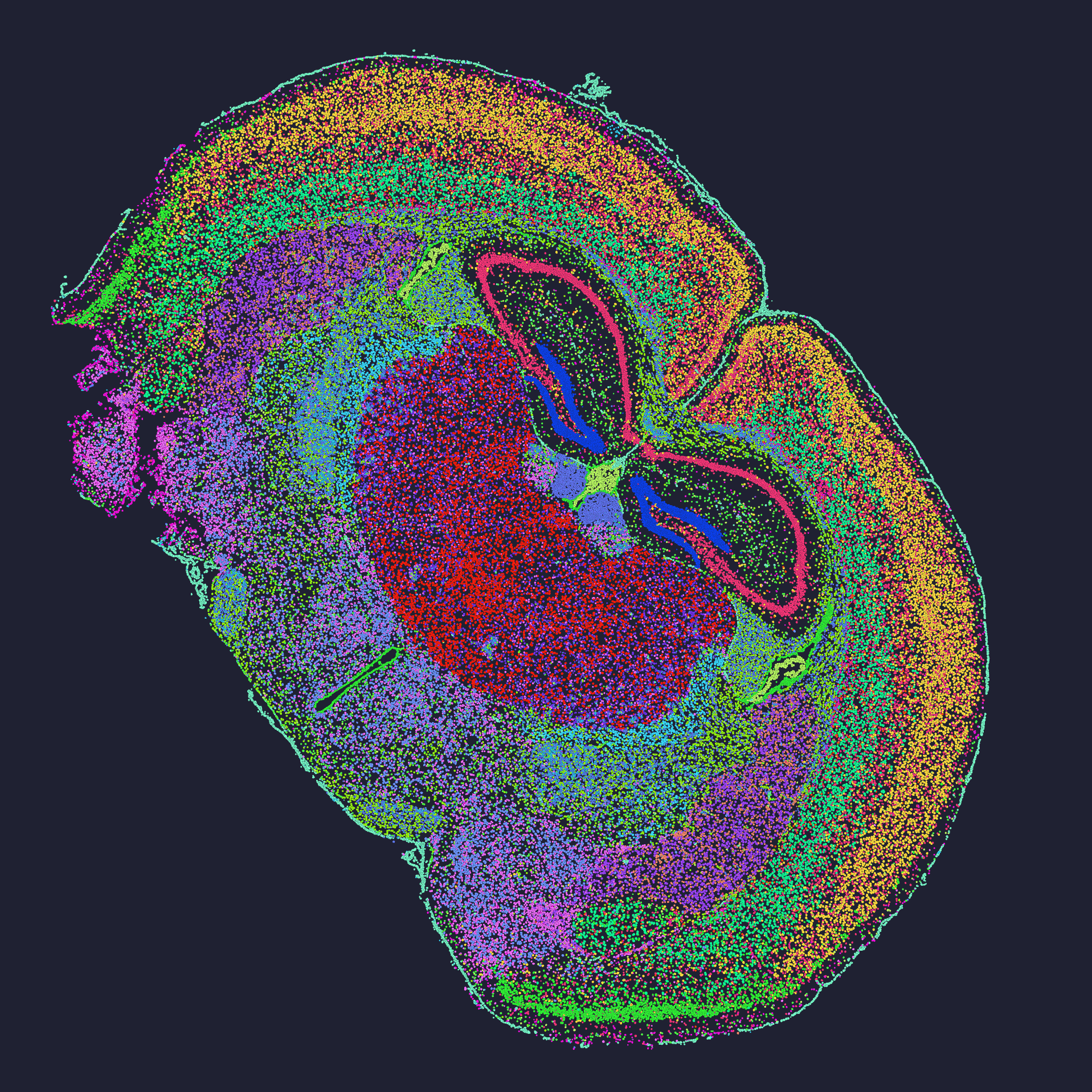
Practical metrics I use when advising labs
I’ve advised three core projects in the last two years where these metrics directly changed the outcome. Here are three concrete evaluation metrics I hand to lab managers: sensitivity (measured as genes detected per spot at a fixed read depth), spatial resolution (µm per feature and the effective cell separation), and scalability (samples processed per week at lab-standard throughput). Use those to compare claims. For example: when a vendor claims “single-cell resolution,” ask for a quantified µm metric and a benchmark dataset run under your RNA quality. I remember a demo where a platform’s advertised resolution didn’t hold once we used FFPE tissue — a costly lesson (we had to rerun six samples). No fluff. Real numbers. Real consequences.
I’m not neutral here; after 17 years working between sequencing facilities and clinical labs, I trust methods that show transparent QC and provide raw read-level diagnostics. If you want to shortlist tools, demand the same three metrics I described. Then pilot on a small set — one discovery slide with high-resolution capture, one broader grid — and measure drop-out. That’s how I avoid wasted runs. One last note — curiosity matters, but so does patience. If you want help interpreting vendor benchmarks, I’ll walk you through them.
For practical resources and to see comparative outputs, check work from stomics — they publish datasets that helped me benchmark a recent pilot run.